MLX-Quantum: Differentiable Quantum Layers on Apple Silicon

For the past year I've been building hybrid quantum neural networks, and one gap kept nagging me: there was no clean way to plug a quantum layer into Apple's MLX. You could drive Qiskit from Python, but every forward and backward pass crossed a slow boundary and ran on the CPU.

So I built mlx-quantum: a differentiable statevector simulator written entirely in MLX. It runs on the Metal GPU, differentiates through MLX's own autodiff, and drops into any model like a normal nn.Module.

📌 The Idea

Instead of connecting MLX to a quantum simulator, I reimplemented the simulator inside MLX.

A statevector is a complex mx.array of shape (batch,) + (2,) * num_qubits.
Gates are einsum contractions over that array.
Because it's all native MLX ops, mx.grad differentiates the circuit directly; no custom gradient code, no NumPy round-trip.

The result: a quantum layer that trains like any other MLX layer.

🧠 Quickstart

QuantumLayer is a trainable mlx.nn.Module. Drop it in and train:

python
import mlx.core as mx
import mlx.nn as nn
from mlx_quantum import QuantumLayer

class HybridMLP(nn.Module):
    def __init__(self):
        super().__init__()
        self.pre = nn.Linear(8, 4)
        self.qnn = QuantumLayer(num_qubits=4, reps=2)   # trainable quantum layer
        self.post = nn.Linear(4, 3)

    def __call__(self, x):
        x = mx.tanh(self.pre(x)) * mx.pi                # encode into rotation angles
        return self.post(self.qnn(x))

The quantum weights are ordinary MLX parameters; nn.value_and_grad and any optimizer update them automatically. No special handling.

🔗 Building Custom Circuits

The simulator primitives are public, so you can build any circuit as a plain differentiable function:

python
from mlx_quantum import zero_state, apply_1q, apply_2q, expval_all_z, H, ry, CX

def circuit(x, weights):            # x: (batch, n) angles, weights: (n,)
    n = x.shape[1]
    state = zero_state(x.shape[0], n)
    for q in range(n):
        state = apply_1q(state, H, q)
    for q in range(n):
        state = apply_1q(state, ry(x[:, q]), q)         # per-sample encoding
    for q in range(n):
        state = apply_1q(state, ry(weights[q]), q)       # trainable
    for q in range(n - 1):
        state = apply_2q(state, CX, q, q + 1)
    return expval_all_z(state)       # <Z> per qubit

grads = mx.grad(lambda w: mx.sum(circuit(x, w)))(weights)  # just works

⚙️ Two MLX Quirks Worth Knowing

Getting this working on Metal meant avoiding two operations MLX can't yet compile for complex arrays:

The initial state is built as a constant, not via in-place assignment and the latter compiles to an unsupported complex GPU scatter.
Gates are contractions, not take/gather, whose backward pass is also a scatter.

These two choices are the reason the whole thing stays GPU-resident and differentiable.

📊 The Results

I validated against Qiskit end-to-end: Statevector for forward values, ReverseEstimatorGradient for gradients.

Speed - MLX vs driving Qiskit's EstimatorQNN from Python:

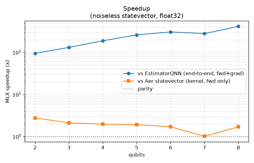Speedup vs qubits

250–1770× faster for small circuits. The chart shows two baselines honestly: the big win is end-to-end (deleting Python orchestration), while against Aer's compiled kernel the forward-only gain is a modest ~2×.

Accuracy - it computes the same numbers:

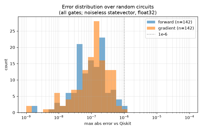Error distribution

Across 142 random circuits covering every gate, forward and gradient errors sit at ~1e-6 with the float32 noise floor. Not cherry-picked.

It trains identically using the same circuit, init, data, and optimizer:

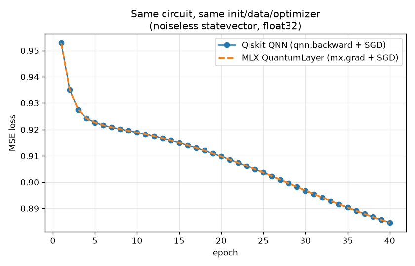Training overlay

The MLX and Qiskit loss curves lie on top of each other. Same learning, a fraction of the time.

✅ Scope & Honest Limits

This is worth being precise about:

Noiseless statevector, float32. No density-matrix / hardware-noise modeling, that's a genuine gap vs Aer.
~26-qubit ceiling. Statevector memory is 2ⁿ; it stays fast to ~24 qubits, then hits the wall hard.
The speedup is mostly deleting the Python boundary, not out-computing Aer's C++ kernel. The two-line chart makes that explicit.

Inside that box, the claim is airtight: same results as Qiskit, dramatically faster, plug-and-play in MLX.

Conclusion

The interesting part wasn't speed for its own sake; it was realizing that once the simulator lives inside MLX, quantum layers stop being special. They're just differentiable functions. mx.grad handles them like anything else, and you train hybrid models with zero connector glue.

Open source (MIT) on GitHub. Runs on Apple Silicon, depends only on MLX and NumPy; Qiskit is optional and used solely to cross-validate.